Getting started¶

Units¶

All length is in cm, densities in g/cm3, energy in MeV.

Usage¶

Several well-documented notebooks will guide you under the Examples. The examples describe how to build simple or more complicated experimental setups, and how to visualize the traveled distance maps, the contribution maps and the geometric efficiency.

In the following, an input of a simple 4x4 assembly is described. The same geometry is used as an example in Working principle. The pins are fuel rods without any cladding (material f) surrounded by water (material w). The example assumes that you have managed to install feign and to obtain some data files after following the instructions at the Installation page.

First, one needs to import the feign modules.

from feign.geometry import *
from feign.blocks import *

Then define the materials with a unique identifier and set their densities and the path of the mass attenuation data.

f=Material('1')
f.set_density(10.5) #g/cm3
f.set_path(('/data/UO2.dat',1))

w=Material('2')
w.set_density(1.0)
w.set_path(('/data/H2O.dat',1))

Then, the pin types can be defined. Each pin has a unique identifier (used later to describe the fuelmap), and with the Pin.add_region() we can create nested annular material regions.

fuel=Pin('1')
fuel.add_region(f,0.5) #cm

Based on the pins we can create a rectangular assembly. This requires to describe the size of the lattice upon initialization, set the lattice pitch size, the source material (or materials), the coolant material (what is around the nested annular regions), and the fuelmap. The elements of the fuelmap are the identifiers used at the definition of Pin() objects. The assembly will be created so that the center of it will be at the origin of the coordinate system.

assy=Assembly(4,4)
assy.set_pitch(1.3)
assy.set_source(f)
assy.set_coolant(w)
assy.set_pins(fuel)

fuelmap=[['1','1','1','1'],
         ['1','1','1','1'],
         ['1','1','1','1'],
         ['1','1','1','1']]

assy.set_fuelmap(fuelmap)

At least one detector point needs to be defined in the problem. Each detector has an identifier, and a location has to be set. A Point() object (from the feign.geometry module) is used for this.

det=Detector('D')
det.set_location(Point(10, -10))

Optinally one may create Collimator() objects and assign them to detectors. Also, one may create Absorber() objects. Then, we have to create an Experiment() objects, and link all the previousl created objects to that.

ex=Experiment()
ex.set_assembly(assy)
ex.set_detectors(det)
ex.set_materials(f,w)

If the user is interested only in the traveled distance maps (as described in Working principle), then the input is done, and the Experiment.Run() method can be called. However, if the geometric efficiency is also of interest, one needs to set energy lines at which the efficiency should be evaluated. The definition is done by a list of strings, because later these are used as keys for the dictionaries storing the pin-wise contribution maps.

elines=['0.6','0.8','1.5','2.0']
ex.set_elines(elines)

We could set optional things, for example the output file to store the geometric efficiency. But at this point everything is set to perform the calculation.

ex.Run()

In this case the source points will be the center of the pins. However, that might not be a valid approximation for many cases. This one can set the number of random source locations per pin. Of course, this will make the computational time longer (the time scales roughly linearly with the number of random sites per pin).

ex.set_random(10)
ex.Run()

Upon running the Experiment.Run() first some checks are done on the Assembly() and Experiment() objects (see in the API docs for assembly and for experiment), which may print warning or error messages if some required parameter or object has not been defined. Assembly.checkComplete() and Experiment.checkComplete() may be run while developing the input, if you are not sure whether something is missing from your input. However, these checks will not provide geometry checking beyond checking that the pin radii are smaller than the assembly pitch. You have to make sure that no absorbers are overlapping with other absorbers or with pins. Experiment.Plot() is plotting the geometry of the experiment (more info here), which might be helpful to check whether there are any overlaps. However, keep in mind that large geometries with a zoomed out view do not render perfectly.

Running the Experiment.Run() method will update a bunch of attributes of the object and fill them with results. The visualisation of these results is shown in the Examples. The main interest is of the mean (over source points) geometric efficiency curve averaged over all detectors, which is stored in Experiment.geomEffAve with its standard deviation Experiment.geomEffAve (non-zero only if Experiment.set_random() is used to set the number of random source points).

Working principle¶

feign implements a 2D point-kernel method to estimate the uncollided point-detector gamma flux around a rectangular spent fuel assembly. The 2D approximation is valid when the fuel assembly is viewed through a horizontally aligned collimator.

After defining an experimental setup with a rectangular fuel assembly placed in the center, the code will iterate through each pin location and trace a ray from the pin towards a detector point. Tracing here means that it will determine how long distance the uncollided ray would travel in various materials.

Let’s consider a simple example as below: there is a 4x4 assembly, the pins are fuel rods without any cladding (material f) surrounded by water (material w). If one draws a line from a pin towards a detector (red circle), some parts of the line are passing through other pins. The code evaluates where are the intersections of the rays with pins (and optionally other absorber elements placed between the detector and the assembly), and determines the total distance traveled in a given material:

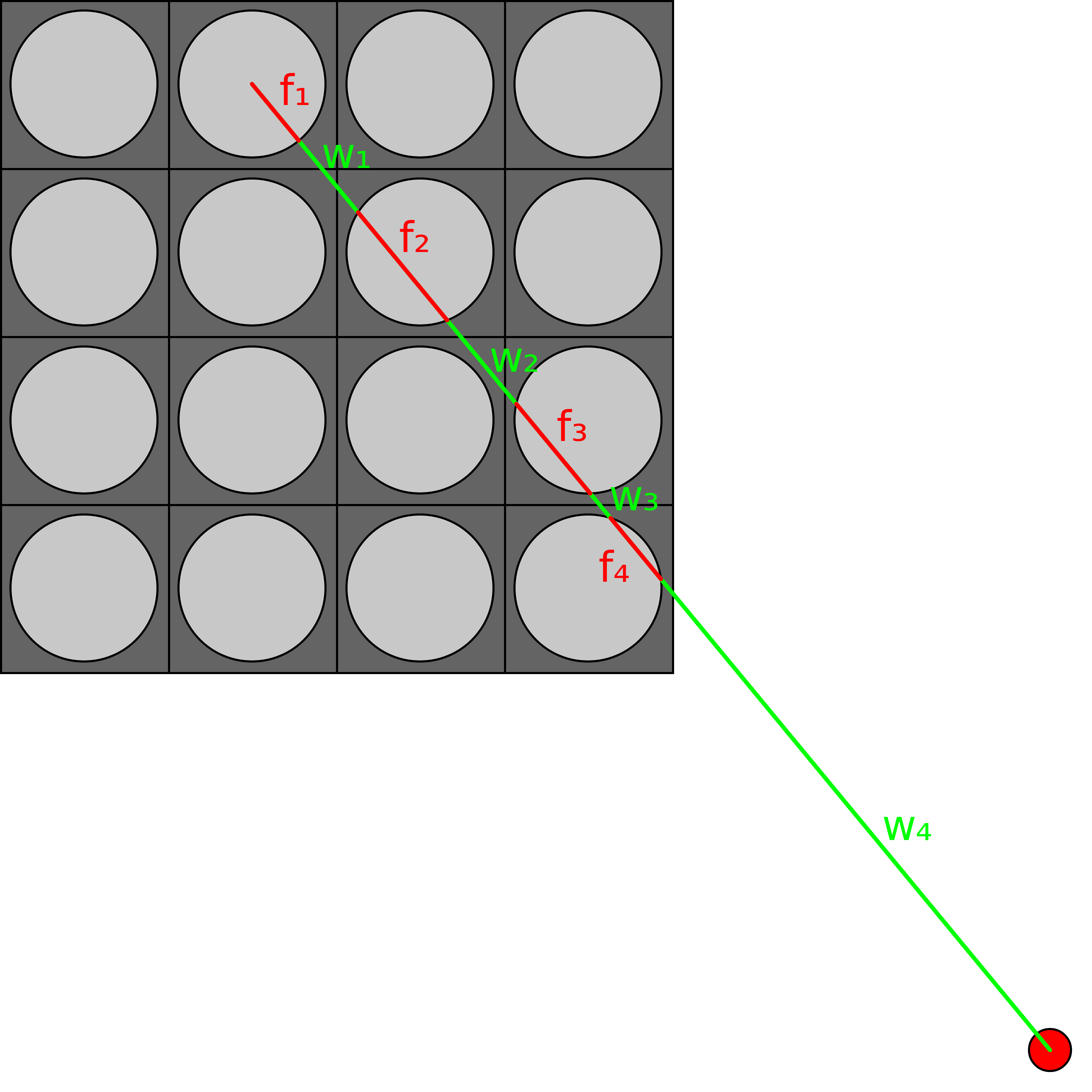
After doing this for each pin, it is possible to build a traveled distance map, which is represented in the code as a dictionary. The keys are material identifiers and the values are matrices describing the pin-wise traveled distance through the given material. Based on these traveled distance maps and on the total attenuation coefficients of the materials, it is possible to compute a contribution map. Contribution here means the probability that a ray emitted from a certain pin will hit the detector, such as

is this probability for each energy \(E\) requested by the user that a gamma-ray emitted from position \(i\) hits the detector without collision. Where \(R_i\) is the distance between the source position and the detector, \(\mu_m\) is the total attenuation coefficient of material \(m\) and \(d_{i,m}\) is the distance traveled by a gamma-ray emitted from position \(i\) through material \(m\). The weight \(w_i\) is the relative emission rate of the given pin (one may consider that pins have different burnup). feign sets this value to 1, however the user can multiply the contribution map with a different weight map (note, that the weight map might depend on the gamma energy as well). In the above example, for the selected pin this probability would be

The average of all these pin-wise probabilities is results in the geometric efficiency (in \(\frac{1}{\rm particle}\) units) of the experimental setup.

However, emitting a ray from the middle of the pin is not necessarily a valid approximation. Thus, feign allows for setting how many random source points should be sampled from each pin. In this case the code is able to calculate an average geometric efficiency and its standard deviation.