Scripts
I am using ENDF-B-VI.8 decay data in Serpent2 depletion calculations. The reason is simply because that is what we have on our cluster. Lately, I wanted to make some studies on air activation next to a neutron generator, and I found that several, possibly important nuclides are not included in the decay data file (eg. N-13, which decays quickly, nevertheless has a quite strong gamma energy, and a nonnegligible amount is produced from N14(n,2n) reactions). So I figured it is time to download newer data. Decay data is available from IAEA, unfortunately not as a neat file how I expected… each nuclide has its info in a separate file, zipped, just in case.
I wrote a quick script, which parses for the links of the zips, unzips them, and puts everything in one .dat file. Later I found there is an index page as well, which would have made the script a bit simpler (no need for the condition to check whether the link ends with ‘zip’), but well, this works.
iaeaurl='https://www-nds.iaea.org/public/download-endf/ENDF-B-VIII.0/decay/'
path='/home/zsolt/Documents/useful_misc/endfdata/'

import requests
r = requests.get(iaeaurl)
data = r.content
data = data.decode('UTF-8')

from bs4 import BeautifulSoup as Soup
html = Soup(data, 'html.parser')
zips=[a['href'] for a in html.find_all('a')]

ziptodown=[]
for z in zips:
    if z[-3:]=='zip':
        ziptodown.append(z)

import zipfile

mainstr=''
for z in ziptodown:
    print('downloading... '+z)
    r = requests.get(iaeaurl+z, allow_redirects=True)
    print('done')
    open(path+z, 'wb').write(r.content)
    zip_ref = zipfile.ZipFile(path+z, 'r')
    zip_ref.extractall(path)
    zip_ref.close()
    endfnuc=open(path+z[:-3]+'dat').read()
    mainstr=mainstr+endfnuc

open('endfdecay.dat','w').write(mainstr)
I did some tests on an infinite PWR depletion problem, to see the impact of the new library. It is actually not negligble. Also, now I will have quite a few new nuclides in my inventories, for example thorium isotopes (L):) Also, I got my stuffs for the air activation study.
I usually find myself becoming quite enthusiastic about something quickly, then looking up tutorials, starting them, and stopping it after a while. Just to give an example, I have much more unfinished coursera courses than finished ones. I guess this behaviour is not characterisitc only for me. Nevertheless, there are some tutorials one “needs” to finish, ones what you actually plan to use on a daily basis. Yesterday I went through Dan Becker’s machine learning tutorial on kaggle. Well, I have an interesting relationship with machine learning and sklearn… I am fiddling around with it almost a year ago now, I did parts of Andrew Ng’s coursera course to help me understand the underlying theory, but then I started using scikit-learn on my own. I think I may haved scrolled through their own tutorial, but it doesn’t require much tutorial to use scikit-learn when you already have an understanding of the implemented methods… Then I got this mail from kaggle that they gonna have some advanced ML course soon, and in order to take it, one should know before hand what is included in the basic course. So well, I figured, maybe it is worth checking what is in the basic course:) Not much new, but still I got couple of more ideas on validating my own models.
Nevertheless, after a while I started to read the number of views on each chapter, and I observed that there is a real decay there. Which was kind of surprising, since this is an extremely short tutorial, literally just few hours. However, the trend nicely coincides with my tendency of not finishing courses as well…:) But of course, kaggle is a platform for machine learning practioners, so maybe many people just opened up the course in hope of learning something new, but then they realized this is really a 101 tutorial, way undert their knowledge, so they quickly left it.
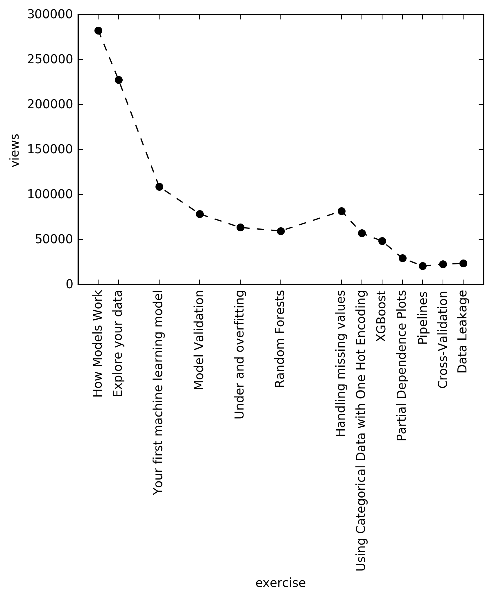
There is a slight bump of at the chapter “handling missing values”, which may be due to the fact, that many people wanna handle missing values, or because that is the first chapter of the Level 2 part, and many people just jumped there after couple of Level 1 chapters. Also, the ticks are farther between some chapters, the reason is, because I did not include the “exercises” between the chapters (no views were easily available for those), however I kept the original index, since maybe some people lost enthusiasm during those parts…:) Also, trend in the number of forks could have been a better representation of the actual decay… Just in case the code behind the plot is below. Values of the views are recorded today (2018. september 14.).
data=[[1, 282405,  'How Models Work'],
[2, 227382,  'Explore your data'],
[4, 108933,  'Your first machine learning model'],
[6, 78478,  'Model Validation'],
[8, 63490,   'Under and overfitting'],
[10, 59584,  'Random Forests'],
[13, 81739,  'Handling missing values'],
[14, 57043,  'Using Categorical Data with One Hot Encoding'],
[15, 48362,  'XGBoost'],
[16, 29441,  'Partial Dependence Plots'],
[17, 20600,  'Pipelines'],
[18, 22662,  'Cross-Validation'],
[19, 23557,  'Data Leakage']]

data=pd.DataFrame(data,columns=['ex','views','exnames'])

ax =plt.subplot()
ax.plot(data.ex,data.views,'ko--')
ax.set_xlabel('exercise')
ax.set_ylabel('views')
ax.set_xticks(data.ex)
ax.set_xticklabels(data.exnames, rotation=90)
plt.savefig('learningdecay.png',dpi=300,bbox_inches='tight')XCOM is “a web database which can be used to calculate photon cross sections for scattering, photoelectric absorption and pair production, as well as total attenuation coefficients, for any element, compound or mixture”. XCOM has a handy web interface to the database and one can quickly generate gamma cross section tables, which can be further used in codes or to compare measurement data. XCOM also has a Fortran code, thus the user can type inputs from the command line. Nevertheless, it doesn’t handle inputs from text files. To be fair, the gamma energies of interest can be read from a file, however (and I really don’t understand the reason), the description of the material composition cannot be read from an input. Some time ago I wanted to investigate the burnup dependence of the total attenuation coefficents of spent nuclear fuel, which would be interesting for an other work. Well, when it comes to spent nuclear fuel, I really didn’t want to type in all the elements, and anyhow I should have done this for various burnups, so manual input typing is no way. Up to now I decided to neglect the effect of burnup on the gamma transport for a while (mainly because of the lack of input for XCOM), but recently we got a master student who was spending few weeks on investigating the same, and it turned out that the total attenuation coefficient depending on the gamma energy decreases with 1-3% between 0 and 110 MWd/kgU burnup. Which is certainly not huge, nevertheless not negligible. The student was using some matlab script called xraymu.m in his work, however since my program, where I need to use these coefficients, is done in python, I would have prefered using XCOM directly from python.
So I decided that I will implement the input reading in the XCOM code. Since it was at least 2 years ago that I used Fortran last time, I kept pushing this task ahead, but today I decided that I will look into the code, find out where to implement the reader and do it. Just in case I googled again (I have done it once before already:)): how to type input in command line with python. Once again I have gotten pygui as a choice (which is powerful, but I used it for some other tasks, and it is slow, you need long pauses to make sure every operation is done, so that is really a last resort for some things, but not for this task), and otherwise the keyword “input” just hijacked the query and pointed me to other topics. So yepp, I swallowed and opened the code, and after 5 minutes of trying to find the right variables around ‘go to’-s and unindented lines, it just hit me all of a sudden… I want to pipeline a sequence of strings (ie the element and their weight fractions) into XCOM, and that’s it. Bash… As Master Foo teaches.
For some ad hoc composition the “script” would look like this
printf 'spentfuel\n4\n2\nH\n0.1\nO\n0.9\n1\n3\n1\n3\n0.6\n0.8\n0.9\nN
        \ntest.out\n1\n' | ./XCOM
#4  - want a composition
#2  - number of components, in this case the composition is 10% H, 90% O
#H
#0.1
#O
#0.9
#1  - accept this
#3  - want own gamma energy list
#1  - typed in from keyboard
#3  - number of lines
#0.6 - in MeV
#0.8
#0.9
#N  - don't save this into file
#test.out - name of the output table
#1 - bye bye
To interface eg. Serpent burnup data with XCOM, basically one only needs to update the string in printf according to the fuel inventory. I may write about that an other time.
I am an enthusiastic swedish learner on Duolingo. It is far not the best way to practice a language, rather just a piece in the puzzle, however most of the days I don’t have time or strength to listen to the swedish radio or read news, and I am really bad at sustaining a conversation in swedish (everybody speaks english, why should I limit myself in experssing my thoughts?). Nevertheless, Duolingo provides a way to force me for a daily practice of few minutes, and at least my vocabulary gets strengthened, which is definitely useful for everyday life in Sweden (reading documents etc). That said, I have a 679 day streak on Duolingo currently, and I am afraid that if I’m loosing it, I will loose my motivation to keep at least these few minutes of daily practice as well. Duolingo has one option to keep up the streak on days, when one cannot do the daily practice: the streak freeze. However, this option gives only one extra day buffer, since one needs to buy a new streak freeze (fortunately, not for real money) after using one. Hence, if the user is unable to login for two consecutive days, the streak is gone. Interestingly, with my soon 2 years long streak, there was only one day when I used a streak freeze (and even that was due to a server failure of Duolingo, when my daily XP didn’t get registered), which seems crazy; this basically means that for 2 years every day I had possibility to login, regardless whether I was travelling somewhere or not.
Since I am planning to go on a longer trip to Mexico, I was wondering what if I won’t be able to login for two days. The chance for that is slim, but still I started to wonder, and anyhow, if not this time, maybe for another trip I can end up in that situation. I know, I know, this is a real first world problem, loosing a duolingo streak, big deal:)
I quickly googled Duolingo API, and luckily in every community nowadays you can find at least one geek, who already provided a solution to your worries. There is an unoffical Duolingo API, which allows you to buy streaks from python. Perfect. It is anyhow worth playing with it, since one can get control over the learnt words etc, so certainly some nice applications could be built around it. However for me the important thing is that with three lines I can buy the streak freeze. Nothing else to do just put the script in crontab to be launched every morning from a computer which will be connected to the network for the days I’m abroad (and make sure that I have enough Duolingo toy-money to purchase the streak, but this doesn’t really concern me).
import duolingo
lingo = duolingo.Duolingo('username',password='*******')
lingo.buy_streak_freeze()
Note: when installing it with $ pip install duolingo-api, some old version gets installed, which does not contain the buy_streak_freeze() method for the Duolingo object, so I would advice downloading the source from the github link above.
Not surprisingly this post is also related to fuel assemblies and their geometries. Namely, I’m planning to give a presentation and I’d like to say few words about the challange in performing Monte Carlo gamma-transport simulations in large fuel assemblies. The main challange is obviously the large amount UO2 between the detector and the source. Nevertheless, this “large amount” varies quite a lot from pin to pin. Clearly, if a detector is facing one of the corners of a 17x17 assembly, then gamma rays emitted towards the detector by the pin in the corner will see on average one pin radius thick UO2 (4.1mm), whereas gamma rays emitted from the opposite corner will see around (16*2+1) pin radius thick UO2 (135.3mm). In my presentation I’d like to give an average thickness, or well, a more reasonable average than (135.3+4.1)/2. So I was thinking about calculating the thickness seen by each pin. Anyhow, the contrubiton made by a pin to the detector signal is related to the this fuel thickness seen by a pin, so this can be a nice quantity to know. And calculating this thickness has to be way easier then estimating the contribution, right?
Ok, let’s do it. Preliminaries: I made some approximations in the geometry compared to a real fuel assembly: I consider only fuel pins in a water-filled lattice (ie. no cladding), the lattice is 17x17, the pitch size is 12.6mm, which makes the assembly 214.2 mm wide. The fuel pins have radii of 4.1mm. I place the origo in the central pin. I consider that every lattice position is filled with fuel (ie. no control rods, to keep the script cleaner). The detector point is 55cm from the origo, facing the upper right corner, ie its location is (388.9,388.9). The fuel is surrounded by water (since I also want to quantify the “water seen” by the pin, this is important). Clearly, the problem has a symmetry, so one can just compute the thicknesses for the upper or the lower triangle (disclaimer, I didn’t do this, since I though run time won’t be a problem).
I actually had two solution to calculate the thickness of the fuel seen. The first one was the lazy way of doing it, and it turned out to be slow as well, so I just quickly summarize it, and at the end of the post I will keep the script anyhow, since it contained some nice ideas. Since I thought, I am lazy to check analytically where a line would cut a circle, my first idea was to do this numerically. That is, I created a mesh over the fuel (in 2D), and when creating the mesh I immedietly kept track of which meshpoint is located in fuel region and which one is in the surrounding water. Then I iterated through the centers of each pin: I draw a line between the pins’ center and the detector point, calculate the slope and the intercept of the line, and then I numerically run through this line, and check whether the given meshpoint is in fuel region or not. If yes, then I will calculate the distance between the current meshpoint on the line and the previous one, and sum it to a variable accounting for the thickness of the fuel seen. One can immedietly see the drawbacks of such solution: 1, One will just estimate this thickness, and the accuracy of the estimation depends on the size amount of mesh points. 2, And still, when the line crosses the boundary between a fuel and water region, one either tries to handle this correctly, or has a bias. 3, The more meshpoints one has, the longer it will take to check whether a meshpoint is in a fuel or water region. Well, in deed I did this, with a meshsize of 0.1 mm, and well, I was actually a bit surprised how slow this is, I assumed this will be slow, but didn’t think this will take hours.
So I finally decided to do this the right way: iterate through the centers of each pin, draw a line between the pins’ center and the detector point, calculate the slope and the intercept of the line, and then iterate through the pins between the detector and the actual pin, and calculate where the line intersects the pins, and sum up the distances between the intersections.
Actually it turns out the this way is way simpler that my first idea. There are two functions which are handy to have.
First the distance between two points
def distance(p1,p2):
    return np.sqrt((p2[0]-p1[0])**2+(p2[1]-p1[1])**2)
Second, the intersections between a line and circle (the line is defined by the slope m and the intercept a, and the circle is defined by the center c and the radius r). Interestingly, I haven’t found a formula after quick googling, so here one can find the quadratic equation after plugging the line equation into the circle equation. One just needs to solve this, and since I don’t care about cases when there is only one intersection (ie the line is a tangent line), I will not return any thing for those case.
def circlelineintersect(m, a, c, r):
    A=1+m**2
    B=(2*(a-c[1])*m-2*c[0])
    C=(c[0]**2+(a-c[1])**2-r**2)
    D = B**2-4*A*C
    if D < 0:
        return []
    elif D == 0:
        return []
    else:
        x1 = (-B+math.sqrt(B**2-4*A*C))/(2*A)
        x2 = (-B-math.sqrt(B**2-4*A*C))/(2*A)
        y1 = a + m*x1
        y2 = a + m*x2
        return [[x1,y1],[x2,y2]]
Finally we can take a look at the

Appendix
Here comes the slow numerical solution. The units are kept as 0.1mm, in order to use integers for coordinates, it is useful, when checking whether a coordinate is in the fuel region. Also, I could have used numpy directly to create a mesh.
import numpy as np
import matplotlib.pyplot as plt
#create mesh geometry goes -12, -12 till something else:)
def distance(p1,p2):
    return np.sqrt((p2[0]-p1[0])**2+(p2[1]-p1[1])**2)

h=1
pitch=126  #1.26 cm, 12.6 mm, 126 0.1mm
p=63
r=41
detx=3889
dety=3889
watercoord=[]
fuelcoord=[]
center=[]
#first create coordinates of grid points
for i in range(-8,9):
    for j in range(-8,9):
        x=i*2*p-p
        y=j*2*p-p
        center=[i*2*p,j*2*p]

        for xi in np.arange(x,x+2*p,h):
            for yi in np.arange(y,y+2*p,h):
                if ((xi-center[0])**2+(yi-center[1])**2)<=r**2:
                    fuelcoord.append([xi,yi])
                else:
                    watercoord.append([xi,yi])
fc=np.array(fuelcoord)
wc=np.array(watercoord)


waterseen=[]
fuelseen=[]
for i in range(-8,9):
    print(i)
    for j in range(-8,9):
        print(j)
        ws=0
        fs=0
        center=[i*2*p,j*2*p]
        slope=(dety-center[1])/(detx-center[0])
        intercept=center[1]-slope*center[0]
        x=[]
        y=[]
        x.append(center[0])
        y.append(center[1])
        while x[-1]<=1071 or y[-1]<=1071:
            x.append(x[-1]+h)
            y.append(round(intercept+slope*x[-1]))
            if [x[-1],y[-1]] in fuelcoord:  #cheating here
                fs=fs+distance([x[-1],y[-1]],[x[-2],y[-2]])
            else:
                ws=ws+distance([x[-1],y[-1]],[x[-2],y[-2]])
        ws=ws+distance([x[-1],y[-1]],[detx,dety])
        waterseen.append(ws)
fuelseen.append(fs)I am running most of my heavy computations on a cluster, which sometimes gets rebooted due to various reasons. This posts summarizes the method to find which computations haven’t been finished yet when the cluster rebooted.
Short background
When I’m creating some synthetic data for multi variate analysis, usually I try to follow some simple pattern to create input names for MCNP (the software I use). In the name I have some tag for the type of the computations (eg. ‘m5’ for MCNP computation with F5 tally), then a tag for the case I’m running (eg. ‘O’ for the original or reference case), and then finally some iteration number. So finally I end up having input file names like ‘m5O115’ and the corresponding MCNP output and run tape file would be ‘m5O115o’ and ‘m5O115r’, respectively.
For running the computations, I have some main python script to iterate through a set of parameters to be modified in the input. This script creates the files in a loop, then connects through ssh to one of the computing nodes on the cluster, runs the computations, exctracts the output, and goes to the next parameter to create the next input etc. Several nodes are available for me, so let’s say I want to run 120 inputs, then I would run the same script slightly modified by changing the name of the node to which I want to connect and by including a conditional (if i=>20 and i<40:). Then, I would run the script 6 times for 6 different nodes and conditions (0-20, 20-40, 40-60, you get it), and since other people may use the nodes as well, the progress of my computations varies from node to node. If the cluster shuts down or reboots, it is not the most pleasant thing to ‘ls’ the folder where the inputs, outputs and run tape files are stored and try to see which inputs were created and which weren’t.
Actual task
So I would see after ‘ls’ a bunch of file names, usually not well ordered, like this:
m5O0 m5O102 m5O105r m5O109o m5O112 m5O115r m5O14r m5O18o m5O21 m5O24r m5O28o m5O31 m5O34r m5O38o m5O4o m5O60r m5O64o m5O68 m5O70r m5O82o m5O86 m5O89r m5O92o m5O9o…
From which I should spot whether m5O37, m5O37o and m5O37r are also there.
Of course I could set the options of ‘ls’ neatly, but who keeps in mind those options? Not me:) And still, my eyes would be filled with tears looking through the list…
Honestly, I have done this two times, and I am not proud of myself. But today I got fed up, so I decided to take that few minutes to write a neat script, and save the tears in case there will be some reboots in future. And actually, this few lines of code demonstrates so nicely why I like to work with python.
import os
import re
path=os.getcwd()
os.chdir(path+'/mcnpf5_files/Orig')

files=os.listdir()
indices=[]
for file in files:
    index=int(re.findall(r'\d+', file)[1])
    if index not in indices:
        indices.append(index)

missing=[i for i in range(120) if i not in indices]
print(missing)
(Note: for the given task actually there were some extra checks needed: check whether for a given index all the three files - ie. input, output, runtape - were created, and if yes check whether the output was actually fully completed, nevertheless I skipped that part here.)
Explanation
There is not much to explain here. Because the code explains itself. Maybe I would only highlight the line
index=int(re.findall(r'\d+', file)[1])So again file can be for example ‘m5O115o’, the regexp will find all the numbers in the string, and gives back [‘5’,’115’], out of which I need the second element (since the first element ‘5’ is irrelevant), what I want to convert into an integer.
I wrote a previous post about creating random defects for MCNP input with a python function. However I don’t necessarily want to have always random defects, sometimes I would like to define given structures in my input. Let say, I am reading a paper, where the authors investigated a given defect scenario, which I would like to include in the computations. The simple solution is to look at the Figure in the given paper, and count it with my fingers, which coordinates are needed to be replaced, then include that in my python function and set only the control rod inserts randomly. This is a tedious task already for one exotic geometry… So I wanted to have a tool which faciliates this. Of course ideally I could write a program, which analyses the included figure and based on the different shades it will tell me where are the dummy rods. The problem, that such tool should be always recalibrated if I come across a new paper and a new structure.
So, instead I was thinking to make a small application where I can just click on the rods, which should be dummies, and get he coordinates. Surely, I still do it manually, but it is way less tedious, then writing the coordinates by hand. And this is much more fun.
Few years back I took a course on Coursera (Introduction to Computational Arts), where the first few tasks were done in Processing. I took the course only for fun, didn’t think that it may help me sometime in my professional life. But now when I started to think about how the application would look like and work, the Processing knowledge immedietly came back to me, and I realized it would be a piece of cake to make it in Processing. Of course now I found that the language evolved quite a bit since I last used it, and most of the help found by google is outdated, so I finally used some mixture of Processing and p5.js, and even I don’t really know when I’m using which one, but I cared only about the end product.
I developed the application on openprocessing.org. Probably the easiest way to discuss how it works is to include it here at the beginning. Nevertheless, the application can be found on here. It is way faster when not embedded, and the embedded version is not able to print the results (which was kind of the goal for me)
Quick overview what is this, and what one can do: as default the app shows a 17x17 PWR assembly structure, grey circles are the fuel pins, and black circles are the control rods. If the user clicks on any of the circles, it becomes red, and the coordinates (from 1 to 289 - that is 17x17) of the selected rods are printed (this is what doesn’t show in the embedded version). Hitting ‘z’ will undo the last selection, and hitting ‘delete’ removes all the selections. I set some default partial defects as well: hitting ‘i’ results in a case when some of the rods in the center region are selected (actually this case motivated the whole tool), ‘e’ belongs to a case when some peripheral rods are selected, ‘c’ belongs to a corner selection, and finally hitting ‘r’ will generate a random defect (same as discussed in the above mentioned post).
So let us just quickly review how a Processing application looks like code-wise: one needs two functions usally: a setup() which sets up the default canvas, and a draw() function, which will bring in any functionality, transients of the canvas etc.
function setup() {
	createCanvas(170*4, 170*4);
	background(255);
	DummyPos=[];
        CrPos=[40,43,46,55,65,88,91,94,97,100,139,142,145,148,151,190,193,196,199,202,225,235,244,247,250];
	k=1;
	for(i=0;i<17;i++){
		for(j=0;j<17;j++){
			fill(100);
			rect(40*i,40*j,40,40);
			fill(200);
			for(jj=0;jj<25;jj++){
				if(CrPos[jj]==k){
					fill(50)
				}
			}
			ellipse(40*i+20,40*j+20,35,35);
			k++;
		}
	}
}Currently, I’m working with methods to identify partial defects in nuclear fuel assemblies. Long story short, partial defect means that some parts of a spent nuclear fuel assembly are removed or replaced with some dummies (may be a steel rod, or a fresh fuel rod), and we are planning to do gamma spectroscopy measurements in order to detect such replacements. Currently, I am running MCNP simulations to compute the gamma particle transport from a spent fuel source. MCNP is a particle transport code, which allows the user to define generic geometries in which the particle transport takes place. Since I have to run a large amount of simulations (for different Burnup and Cooling times of the spent fuel), I usually use python to script my MCNP inputs and code calls.
I would like to run simulations for random partial defect patterns in 17x17 type PWR assemblies. In MCNP the user can define “universes” (which basically mean well defined structures, which one can fill to any container, these facilitate the definition of repeated structures). In my case the fuel rods are assigned with universe “1”, the dummy rods are “2”, and the control rod positions are either “4” or “6” (depending whether the control rod is inserted or not in that position). Then in the MCNP input one needs to define the pin-wise structure of the assembly. For example for an assembly, which contains 25 control rod positions which are randomly inserted or not inserted (the location of these positions is defined by the manufacturer) and 17x17-25 fuel pins, the related part of the input would look like this:
     1 1 1 1 1 1 1 1 1 1 1 1 1 1 1 1 1
     1 1 1 1 1 1 1 1 1 1 1 1 1 1 1 1 1
     1 1 1 1 1 4 1 1 6 1 1 6 1 1 1 1 1
     1 1 1 4 1 1 1 1 1 1 1 1 1 4 1 1 1
     1 1 1 1 1 1 1 1 1 1 1 1 1 1 1 1 1
     1 1 4 1 1 6 1 1 6 1 1 6 1 1 4 1 1
     1 1 1 1 1 1 1 1 1 1 1 1 1 1 1 1 1
     1 1 1 1 1 1 1 1 1 1 1 1 1 1 1 1 1
     1 1 4 1 1 4 1 1 6 1 1 4 1 1 6 1 1
     1 1 1 1 1 1 1 1 1 1 1 1 1 1 1 1 1
     1 1 1 1 1 1 1 1 1 1 1 1 1 1 1 1 1
     1 1 6 1 1 6 1 1 6 1 1 4 1 1 6 1 1
     1 1 1 1 1 1 1 1 1 1 1 1 1 1 1 1 1
     1 1 1 4 1 1 1 1 1 1 1 1 1 4 1 1 1
     1 1 1 1 1 4 1 1 4 1 1 6 1 1 1 1 1
     1 1 1 1 1 1 1 1 1 1 1 1 1 1 1 1 1
     1 1 1 1 1 1 1 1 1 1 1 1 1 1 1 1 1
Now, I wanted to have a python function which can create such strings what I can later replace into some reference input file. This in itself is not a huge task, nevertheless I wanted to write up this post, because it is going to be a prerequisite for a coming post. I define the positions of each pin with one number (from 1 to 289 -that is 17X17-, logically as one would read from left to right and then jump to the next row). The function below calculates the number of pins to be replaced with dummies from the size of the defect (given as an input in percentage), then creates a list to hold all the possible fuel rod positions (based on the 25 given control rod positions). Then it creates a random sample of these positions with random.sample() (keep in mind that the python2 version of this function requires an integer as the size of the random subset), then finally it builds up a string to match the above given input structure (the control rod insert is decided with random.choice()).
def createRandomDefect(perc):
    #universe numbers:
    #1: Fuel
    #2: Dummy
    #4: CR Insert
    #6: CR Guide
    import random
    import math
    ND=int(math.ceil((17*17-25)*(perc/100.0))) #number of dummies int() is needed for python2
    SubAsStr=''
    CrPos=[40,43,46,55,65,88,91,94,97,100,139,142,145,148,151,190,193,196,199,202,225,235,244,247,250]
    FuelPos=[]
    for i in range(17*17):
        j=i+1
        if j not in CrPos:
            FuelPos.append(j)
    DummyPos=random.sample(FuelPos,ND)
    col=1
    for i in range(17*17):
        j=i+1
        if col==1:
            SubAsStr=SubAsStr+'        '
        if j in CrPos:
            SubAsStr=SubAsStr+' '+str(random.choice([4,6]))
        elif j in DummyPos:
            SubAsStr=SubAsStr+' '+str(2)
        else:
            SubAsStr=SubAsStr+' '+str(1)
        if col==17:
            SubAsStr=SubAsStr+'\n'
            col=0
        col=col+1
    SubAsStr=SubAsStr[:-1]

    return SubAsStr,17*17-25-ND   #N of source pins
Usage is straightforward:
pattern,NRod=createRandomDefect(30)
print(pattern)
1 2 1 1 1 1 2 2 1 1 2 2 1 2 1 2 1
1 1 2 1 1 1 2 2 1 1 2 1 1 1 1 1 1
2 1 1 2 1 6 2 1 6 2 1 4 1 1 1 1 1
2 1 1 4 2 2 1 2 1 1 1 1 2 4 2 1 1
1 1 2 1 2 1 1 1 1 1 1 1 1 1 2 1 1
1 1 6 2 1 4 1 1 4 2 1 6 1 1 6 1 1
2 1 1 2 2 2 1 1 1 1 1 2 1 2 2 2 2
2 1 1 1 1 1 2 2 1 1 1 1 1 1 1 1 1
2 2 6 1 1 4 1 2 6 1 1 6 1 1 6 1 1
1 2 1 1 2 1 2 1 1 2 1 1 1 2 2 1 2
1 1 1 2 1 1 2 1 1 1 2 1 1 1 1 1 2
2 2 4 1 1 6 2 1 6 2 1 6 2 1 4 1 1
2 1 1 1 1 1 1 1 1 1 1 2 1 2 1 2 1
1 2 2 6 2 1 1 1 1 1 1 1 1 6 1 2 1
1 1 1 1 1 4 1 2 4 1 1 6 1 2 1 1 2
1 1 1 1 2 1 1 1 1 1 2 2 2 1 2 2 1
2 1 1 1 2 1 1 2 1 1 2 1 1 2 1 2 1